Length-weight analysis • mustelus

Background

Length and weight are perhaps the two most routinely taken measurements in fisheries science, although length is the far easier one to measure. Length can be measured quickly and is more commonly the standard measurement, especially for chondrichthyans. Weight is far more challenging to collect, especially in the field. It needs a stable platform and, if at sea, a compensating balance to accurately measure. Weight also varies with gut fullness, body condition, and gonad state. In the case of larger chondrichthyan species, it is often impractical to measure adult animals that weight hundreds or thousands of kilograms. For these reasons, good quality length weight relationships don’t exist for that many chondrichthyan species which is precisely why this information is still worth collecting.

This conversion between length and weight underpins a considerable amount of subsequent work in quantitative fisheries science. Catch is reported and managed in tonnes whereas biological sampling is usually done in numbers of fish at length, so moving between the two requires a weight–length relationship, as does converting population length structure (the distribution of lengths in a population) to biomass. The age-structured population dynamics models that are commonly used in stock assessments need weight-at-age, which is normally obtained by passing predicted length-at-age from a growth curve through the weight–length relationship; yield-per-recruit, spawning stock biomass and other demographic calculations follow. The same relationship underlies body condition indices, which compare the observed weight of an individual against the weight expected for its length (Froese, 2006).

Despite its importance, the length weight relationship is considered trivial, as noted by Froese (2006) who quotes Quantitative Fisheries Stock Assessment (Hilborn and Walters, 2001): length–weight analysis is “a good thing to have your teenage children do” as a way of learning about correlation and regression, and if the teenager struggles with estimating $\beta$ , one can take comfort in assuming $\beta = 3$ .

The relationship between body mass and length in fishes is typically described by a power curve:

$W_i = \alpha L_i^{\beta}$

where $W_i$ and $L_i$ are the weight and length of individual $i$ , and $\alpha$ and $\beta$ are estimated parameters. Individual variability in weight also increases with length, so a multiplicative rather than additive error structure is more appropriate:

$W_i = \alpha L_i^{\beta} e^{\epsilon}, \quad \epsilon \sim N(0, \sigma^2)$

Upon log-transformation this becomes a standard linear regression:

$\ln(W_i) = \ln(\alpha) + \beta \cdot \ln(L_i) + \epsilon$

where $\ln(\alpha)$ is the intercept and $\beta$ is the slope. This is the model fitted by len_weight(), which reports $\alpha$ as a and $\beta$ as b.

Interpreting the parameters

$\beta$ , the exponent, is the more informative of the two parameters. It describes how weight scales with length:

$\beta = 3$ — isometric growth. Weight rises as the cube of length, so body shape and specific gravity stay constant as the animal grows and a fish that doubles in length becomes eight times heavier (i.e. the cube law).
$\beta > 3$ — positive allometry. Large individuals are relatively heavier for their length, gaining girth or depth faster than length.
$\beta < 3$ — negative allometry. Large individuals are relatively more slender for the length.

Froese’s (2006) meta-analysis of 3929 relationships across 1773 species found a median $\beta$ of 3.03, significantly greater than 3, so a slight tendency toward positive allometry is the norm rather than the exception. Froese (2006) indicates that $2.5 < \beta < 3.5$ is the expected range for this coefficient.

$\alpha$ , the coefficient, is the intercept on the log scale and reflects body form: at a given $\beta$ , eel-like and elongate species carry smaller values than fusiform and deep-bodied species. It is also important to note that $\alpha$ depends on the measurement units and on which length measurement was used, changing by a factor of $10^{\beta}$ when length is converted from millimetres to centimetres. Values are therefore not comparable across studies unless the units are the same. Froese (2006) provides some of these commonly used conversion factors.

Bias correction

A subtle consequence of log-transforming in the regression of weight against length is that back-transforming predictions gives the median weight at a given length, not the mean. For a lognormal distribution, the mean is:

$E[W \mid L] = e^{\hat{\mu} + \sigma^2/2}$

where $\sigma^2$ is the residual variance. len_weight() accounts for this — all predicted values and intervals are corrected for back-transformation bias, following Beauchamp and Olson (1973).

The size of the correction is $e^{\sigma^2/2}$ , so it depends only on the residual variance and is constant across the length range. It is negligible for a tight relationship and grows quickly once residual variation is substantial: at $\sigma = 0.1$ it inflates predictions by 0.5%, at $\sigma = 0.3$ by 4.6%, and at $\sigma = 0.5$ by 13%. Reported values of $\sigma$ therefore indicate how much difference the correction makes for a given data set.

Basic usage

library(mustelus)
#> Welcome to mustelus package
data(spottail)

lw <- len_weight(wgt, length, data = spottail)
summary(lw)
#> # A tibble: 1 × 8
#>          a Std.Error.range      b Std.Error Sigma    LL     n len.range 
#>      <dbl> <chr>            <dbl> <chr>     <dbl> <dbl> <int> <chr>     
#> 1 2.13e-10 ( 1.441 - 3.16 )  3.47 ( 0.057 ) 0.102  166.   192 478 - 1301

The summary table reports: the intercept on the natural scale ( $a = e^{\ln(\alpha)}$ ), its standard error range, the slope $b$ , its standard error, the residual standard deviation $\sigma$ , the log-likelihood, sample size, and length range.

In the case of the spot-tail data the exponent, 3.47, is well above 3 and sits near the top of Froese’s expected range, indicating positive allometry: larger spottail sharks are relatively heavier for their length than smaller ones. And a is around 2.1e-10. This value corresponds to the median weight in kilograms of a one millimetre long shark, extrapolated from a curve fitted to individuals two to three orders of magnitude larger, so it doesn’t have any particularly important biological interpretation.

Grouping by sex

Pass a grouping variable to fit separate models per group. A pooled model across all groups is automatically included.

lw_sex <- len_weight(wgt, length, sex, data = spottail)
#> The categorical variable sex has 2 levels.
summary(lw_sex)
#> # A tibble: 3 × 8
#>          a Std.Error.range       b Std.Error  Sigma    LL     n len.range 
#>      <dbl> <chr>             <dbl> <chr>      <dbl> <dbl> <int> <chr>     
#> 1 2.13e-10 ( 1.441 - 3.16 )   3.47 ( 0.057 ) 0.102  166.    192 478 - 1301
#> 2 1.12e-10 ( 0.618 - 2.037 )  3.56 ( 0.086 ) 0.0968  91.7    99 691 - 1301
#> 3 4.47e-10 ( 2.457 - 8.148 )  3.36 ( 0.087 ) 0.107   76.9    93 478 - 1139

Plotting

plot() returns a named list of ggplot objects — one per group — which can be customised with standard ggplot2 calls. The solid line is the predicted mean, the dashed ribbon the 95% confidence interval, and the dotted ribbon the 95% prediction interval. The fits for females and males are shown in Figure 1 and Figure 2.

p <- plot(lw_sex)
p$f + xlab("Total length (mm)") + ylab("Weight (kg)")

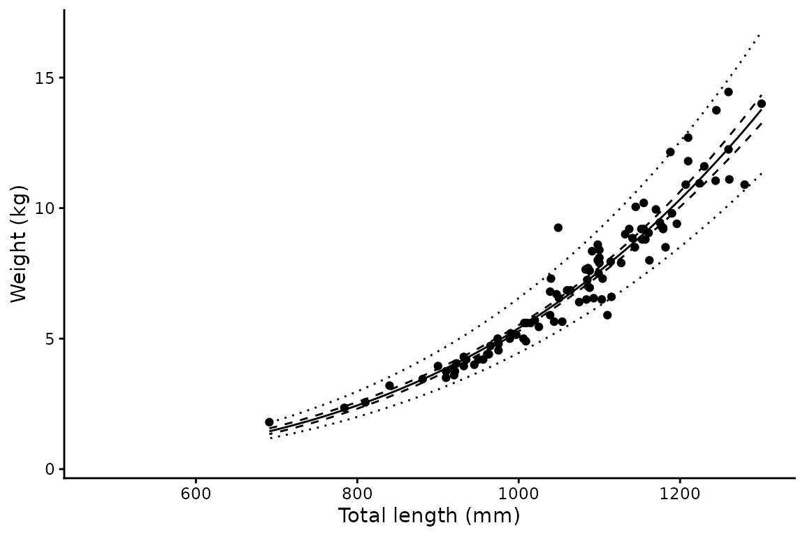
Figure 1. Weight against total length for female spot-tail sharks. The solid line is the predicted mean weight, corrected for back-transformation bias, the dashed ribbon the 95% confidence interval and the dotted ribbon the 95% prediction interval.

p$m + xlab("Total length (mm)") + ylab("Weight (kg)")

Figure 2. Weight against total length for male spot-tail sharks, with lines as in Figure 1.

Confidence vs prediction intervals

Both interval types appear in the output. They answer different questions:

Confidence interval — uncertainty in the mean weight at a given length. Narrows with more data.
Prediction interval — expected spread of individual weights at a given length. Reflects the biological variability captured by $\sigma$ and does not narrow appreciably with more data.

For most fisheries reporting purposes the prediction interval is more informative, as it describes the range of weights you would expect to observe in the field.

Using other length measurements

The function accepts any positive numeric predictor — fork length, precaudal length, or any other measurement that makes biological sense to log-transform.

lw_fl <- len_weight(wgt, FL, data = spottail)
summary(lw_fl)
#> # A tibble: 1 × 8
#>               a Std.Error.range       b Std.Error  Sigma    LL     n len.range 
#>           <dbl> <chr>             <dbl> <chr>      <dbl> <dbl> <int> <chr>     
#> 1 0.00000000249 ( 1.782 - 3.485 )  3.22 ( 0.05 )  0.0940  172.   181 358 - 1015

Output structure

The result is a nested tibble with one row per group. List columns data, coefs, preds, and mods are named by group level for direct access:

# Fitted lm object for females
lw_sex$mods[["f"]]
#> 
#> Call:
#> lm(formula = log(weight) ~ log(length), data = data)
#> 
#> Coefficients:
#> (Intercept)  log(length)  
#>      -22.91         3.56

# Predicted values for the pooled group
head(lw_sex$preds[["all"]])
#>   length    weight    clower    cupper    plower    pupper
#> 1    478 0.4184922 0.3842572 0.4557772 0.3362275 0.5208845
#> 2    479 0.4215356 0.3871409 0.4589861 0.3387031 0.5246255
#> 3    480 0.4245948 0.3900401 0.4622108 0.3411916 0.5283856
#> 4    481 0.4276697 0.3929549 0.4654514 0.3436931 0.5321648
#> 5    482 0.4307604 0.3958853 0.4687079 0.3462076 0.5359633
#> 6    483 0.4338670 0.3988315 0.4719803 0.3487351 0.5397810

The preds data frame contains six columns: length, weight (bias-corrected mean), clower/cupper (95% confidence interval), and plower/pupper (95% prediction interval).

References

Beauchamp, J.J. and Olson, J.S. (1973) Corrections for bias in regression estimates after logarithmic transformation. Ecology 54(6), 1403–1407. doi:10.2307/1934208

Froese, R. (2006) Cube law, condition factor and weight–length relationships: history, meta-analysis and recommendations. Journal of Applied Ichthyology 22(4), 241–253. doi:10.1111/j.1439-0426.2006.00805.x

Hilborn, R. and Walters, C.J. (2001) Quantitative Fisheries Stock Assessment: Choice, Dynamics and Uncertainty. Kluwer Academic Publishers, Boston. (Cited in Froese, 2006.)