Fecundity analysis • mustelus

Background

Fecundity in chondrichthyans — the number of in utero embryos carried by a gravid female — typically increases with maternal body size. fecundity() fits the simplest description of that relationship, an ordinary linear regression:

$F_i = a + b \cdot L_i + \epsilon, \quad \epsilon \sim N(0, \sigma^2)$

where $F_i$ is the number of embryos carried by female $i$ and $L_i$ is her length (or age). The slope $b$ is the increase in litter size per unit length, and is usually the quantity of interest.

Non-gravid animals are excluded

A fecundity count of zero means an animal was not gravid, not that its fecundity was zero. Including such records would bias the intercept downwards and inflate the slope. fecundity() therefore drops records with zero or negative counts before fitting and reports how many were removed. Predictions span the length or age range of gravid animals only.

Basic usage

library(mustelus)
#> Welcome to mustelus package
data(spottail)

fec <- fecundity(emb, length, data = spottail)
summary(fec)
#> # A tibble: 1 × 11
#>       a a.Std.Error       b b.Std.Error r.squared  p.value Sigma     n mean.fec
#>   <dbl> <chr>         <dbl> <chr>           <dbl>    <dbl> <dbl> <int>    <dbl>
#> 1 -7.75 ( 1.24 )    0.00946 ( 0.00108 )     0.527 7.97e-13 0.682    71     3.06
#> # ℹ 2 more variables: fec.range <chr>, x.range <chr>

The summary reports the intercept $a$ and slope $b$ with their standard errors, the coefficient of determination, the p-value for the slope, the residual standard deviation $\sigma$ , sample size, mean and range of observed fecundity, and the predictor range over which the model applies.

Plotting

plot() returns a ggplot object, which can be customised with standard ggplot2 calls. In Figure 1 the solid line is the fitted mean, the dashed ribbon the 95% confidence interval, and the dotted ribbon the 95% prediction interval — the presentation used by Walker (2005).

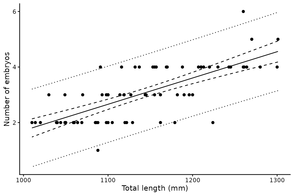
plot(fec) + xlab("Total length (mm)") + ylab("Number of embryos")

Figure 1. Number of embryos against maternal total length for gravid spot-tail sharks. The solid line is the fitted mean, the dashed ribbon the 95% confidence interval and the dotted ribbon the 95% prediction interval.

As in len_weight(), the two interval types answer different questions. The confidence interval describes uncertainty in mean litter size at a given length and narrows as data accumulate; the prediction interval describes the spread of litter sizes you would expect to observe in individual females, and does not narrow appreciably. For predicting the reproductive output of a female of known size, the prediction interval is the relevant one.

Using age as the predictor

Any continuous predictor works — here maternal age rather than length:

fec_age <- fecundity(emb, age_agree, data = spottail)
summary(fec_age)
#> # A tibble: 1 × 11
#>       a a.Std.Error     b b.Std.Error r.squared  p.value Sigma     n mean.fec
#>   <dbl> <chr>       <dbl> <chr>           <dbl>    <dbl> <dbl> <int>    <dbl>
#> 1  1.73 ( 0.303 )   0.227 ( 0.0487 )      0.299 0.000023 0.829    53     3.04
#> # ℹ 2 more variables: fec.range <chr>, x.range <chr>

The fitted relationship is shown in Figure 2.

plot(fec_age) + xlab("Age (years)") + ylab("Number of embryos")

Figure 2. Number of embryos against maternal age for gravid spot-tail sharks, with lines as in Figure 1.

Output structure

Unlike len_weight() and maturity(), fecundity() fits a single model and takes no grouping variable. The result is a one row tibble whose list columns hold the components of that fit:

# Fitted lm object
fec$mods[[1]]
#> 
#> Call:
#> lm(formula = fec ~ x, data = new)
#> 
#> Coefficients:
#> (Intercept)            x  
#>   -7.752597     0.009465

# Predicted values
head(fec$preds[[1]])
#>          x      fec   clower   cupper    plower   pupper
#> 1 1010.000 1.806733 1.479740 2.133726 0.4080167 3.205450
#> 2 1011.462 1.820574 1.496316 2.144831 0.4224940 3.218653
#> 3 1012.925 1.834414 1.512885 2.155943 0.4369645 3.231863
#> 4 1014.387 1.848254 1.529445 2.167063 0.4514282 3.245080
#> 5 1015.849 1.862094 1.545998 2.178191 0.4658851 3.258304
#> 6 1017.312 1.875935 1.562542 2.189327 0.4803351 3.271534

The preds data frame contains six columns: x, fec (predicted mean), clower/cupper (95% confidence interval), and plower/pupper (95% prediction interval).

Reference

Walker, T.I. (2005) Reproduction in fisheries science. In: Hamlett, W.C. (ed) Reproductive Biology and Phylogeny of Chondrichthyes.