Analyse fecundity as a function of length or age

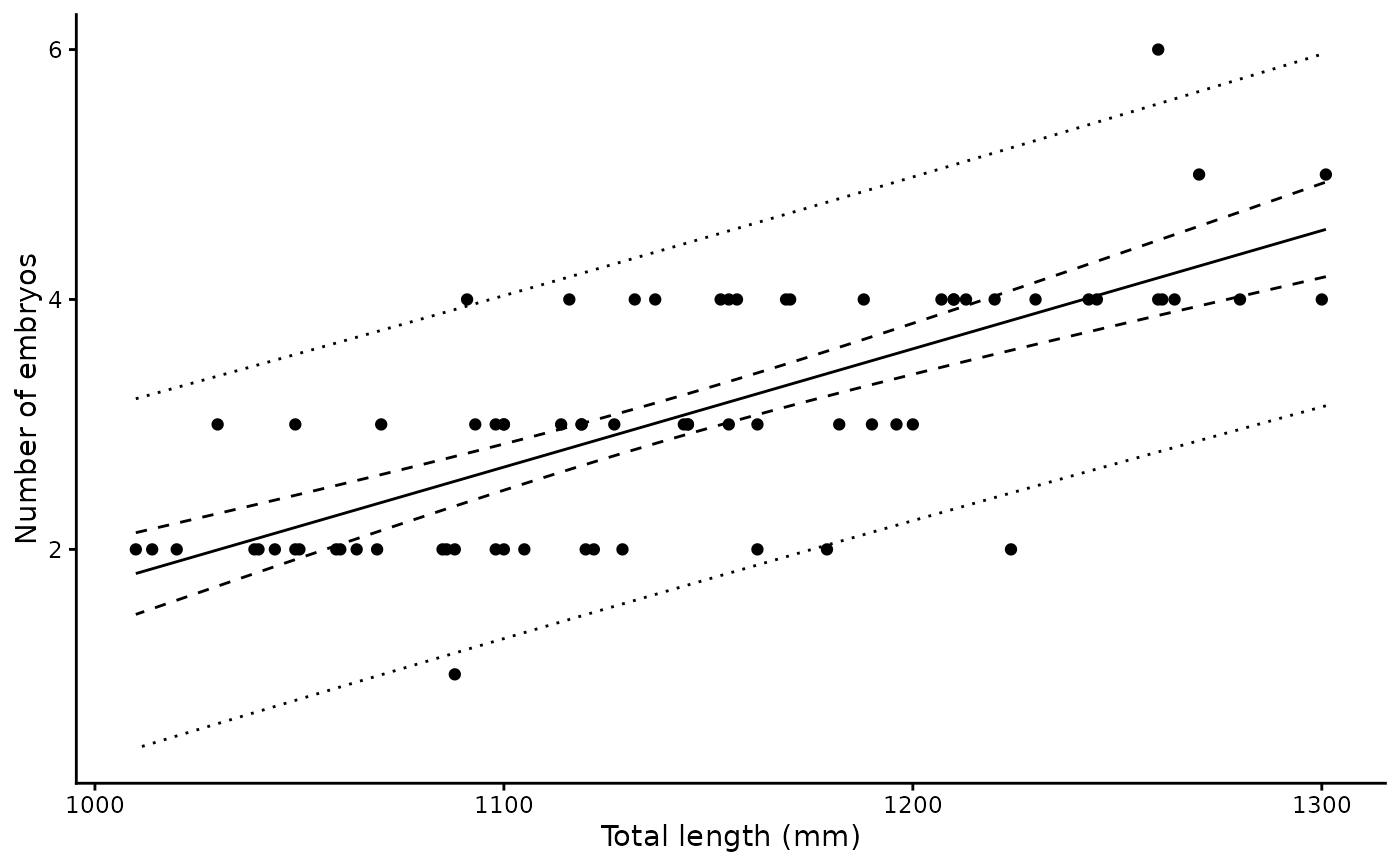
Fits a linear regression of fecundity (e.g. number of in utero embryos) against a continuous predictor such as length or age. Essentially a wrapper for lm() and predict.lm() that tabulates useful summary statistics and returns the predicted mean with 95 percent confidence and prediction intervals, in the style of Walker (2005).

Usage

fecundity(fec, x, data)

Arguments

fec

Numeric vector of fecundity counts (e.g. number of embryos)

x

Continuous predictor variable (e.g. length, age)

data

A data frame containing the above variables

Value

A one row tibble of class "fecundity" containing the list columns data, coefs, preds, and mods.

Details

Records with zero or negative fecundity are dropped before fitting, since a count of zero indicates a non-gravid animal rather than a fecundity of zero. The number dropped is reported as a message. Predictions therefore span the length or age range of gravid animals only.

References

Walker, T.I. (2005) Reproduction in fisheries science. In: Hamlett, W.C. (ed) Reproductive Biology and Phylogeny of Chondrichthyes.

Examples

library(ggplot2)
data(spottail)

fec <- fecundity(emb, length, data = spottail)

summary(fec)
#> # A tibble: 1 × 11
#>       a a.Std.Error       b b.Std.Error r.squared  p.value Sigma     n mean.fec
#>   <dbl> <chr>         <dbl> <chr>           <dbl>    <dbl> <dbl> <int>    <dbl>
#> 1 -7.75 ( 1.24 )    0.00946 ( 0.00108 )     0.527 7.97e-13 0.682    71     3.06
#> # ℹ 2 more variables: fec.range <chr>, x.range <chr>

plot(fec) + xlab("Total length (mm)") + ylab("Number of embryos")