Clasper length analysis

Background

Male chondrichthyans undergo a rapid elongation and calcification of the claspers as they mature. Clasper length plotted against body length or age is therefore sigmoid: near-constant in juveniles, steeply increasing through maturation, and asymptotic in adults. clasp_length() fits that curve:

$$CL = b + (a - b)\left(1 + e^{-\log(19)\,(x - L_{50})/(L_{95} - L_{50})}\right)^{-1}$$

where $b$ and $a$ are the juvenile and adult asymptotes, and $L_{50}$ and $L_{95}$ are the values of the predictor at which clasper length reaches 50% and 95% of the way between them. The $\log(19)$ term is what makes $L_{50}$ and $L_{95}$ mean exactly that — the same reparameterisation used by maturity(), so the two are directly comparable.

The model is fitted on the log scale by nls(). This gives multiplicative error, matching the way variability in clasper length grows with clasper size, and means the fitted curve describes median clasper length at a given size.

Basic usage

Females have no clasper measurement and are dropped automatically, so the whole data frame can be passed in:

library(mustelus)
#> Welcome to mustelus package
data(spottail)

cl <- clasp_length(clasp_length, length, clasp_calc, data = spottail, times = 200)
#> The calcification variable clasp_calc has 3 levels.
summary(cl)
#> # A tibble: 1 × 15
#>       a a_lower a_upper     b b_lower b_upper   L50 L50_lower L50_upper   L95
#>   <dbl>   <dbl>   <dbl> <dbl>   <dbl>   <dbl> <dbl>     <dbl>     <dbl> <dbl>
#> 1  80.2    78.4    82.5  13.1    10.9    15.2  898.      888.      909.  992.
#> # ℹ 5 more variables: L95_lower <dbl>, L95_upper <dbl>, Sigma <dbl>, n <int>,
#> #   x.range <chr>

Claspers are around 13 mm in juveniles and asymptote near 80 mm in adults, with the transition centred on 898 mm.

Plotting

plot(cl) + xlab("Total length (mm)") + ylab("Clasper length (mm)")

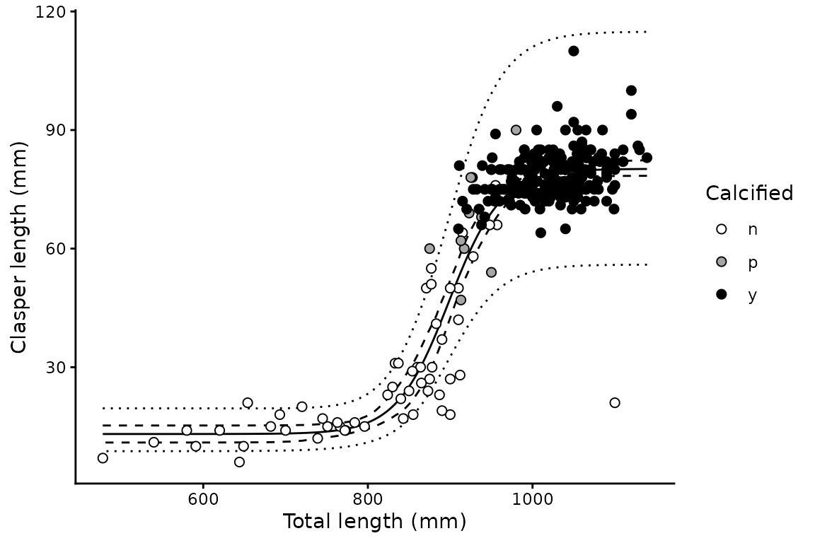
Figure 1. Clasper length against total length for male spot-tail sharks. The solid line is the fitted median, the dashed ribbon the 95% confidence interval and the dotted ribbon the 95% prediction interval. Points are shaded by calcification stage: white, uncalcified; grey, partially calcified; black, fully calcified.

In Figure 1 the solid line is the fitted median, the dashed ribbon the 95% confidence interval and the dotted ribbon the 95% prediction interval. Both are obtained by bootstrap: the confidence interval from the percentiles of the resampled curves, and the prediction interval by combining that bootstrap variance with the residual variance of the fit.

Passing the optional calcification variable shades the points by stage — white for uncalcified, grey for partially calcified and black for fully calcified. This is a useful check on the fitted curve, since the three stages should separate along it: uncalcified animals on the lower asymptote, partially calcified animals through the steep transition, and calcified animals on the upper asymptote. Calcification is used only for plotting and does not enter the model.

Using age as the predictor

cl_age <- clasp_length(clasp_length, age_agree, clasp_calc, data = spottail, times = 200)
#> The calcification variable clasp_calc has 3 levels.
#> 1 of 200 bootstrap replicates failed to converge and were dropped.
summary(cl_age)
#> # A tibble: 1 × 15
#>       a a_lower a_upper     b b_lower b_upper   L50 L50_lower L50_upper   L95
#>   <dbl>   <dbl>   <dbl> <dbl>   <dbl>   <dbl> <dbl>     <dbl>     <dbl> <dbl>
#> 1  82.1    78.4    84.5  10.7    5.31    15.0  1.99      1.81      2.10  3.09
#> # ℹ 5 more variables: L95_lower <dbl>, L95_upper <dbl>, Sigma <dbl>, n <int>,
#> #   x.range <chr>

The fitted curve is shown in Figure 2.

plot(cl_age) + xlab("Age (years)") + ylab("Clasper length (mm)")

Figure 2. Clasper length against age for male spot-tail sharks, with lines and shading as in Figure 1.

Starting values

nls() needs starting values, and clasp_length() derives them from the data: the asymptotes from the mean clasper length of the smallest and largest 20% of animals, and $L_{50}$ and $L_{95}$ by interpolating binned means. Fitting uses the "port" algorithm with both asymptotes constrained positive, since a negative asymptote would make the log-scale model undefined.

If a fit fails to converge, supply starting values directly:

clasp_length(clasp_length, length,
  data = spottail, times = 50,
  start = list(a = 80, b = 13, L50 = 900, L95 = 990)
) |> summary()
#> # A tibble: 1 × 15
#>       a a_lower a_upper     b b_lower b_upper   L50 L50_lower L50_upper   L95
#>   <dbl>   <dbl>   <dbl> <dbl>   <dbl>   <dbl> <dbl>     <dbl>     <dbl> <dbl>
#> 1  80.2    78.1    81.7  13.1    10.7    15.4  898.      889.      909.  992.
#> # ℹ 5 more variables: L95_lower <dbl>, L95_upper <dbl>, Sigma <dbl>, n <int>,
#> #   x.range <chr>

Comparison with maturity

Because both functions report $L_{50}$ on the same scale, clasper elongation can be compared directly with the onset of maturity:

mat <- maturity(maturity_stage, length, data = spottail[spottail$sex == "m", ],
                times = 200)

data.frame(
  quantity = c("Clasper elongation", "Maturity"),
  L50      = c(summary(cl)$L50, summary(mat)$L50),
  L95      = c(summary(cl)$L95, summary(mat)$L95)
)
#>             quantity   L50   L95
#> 1 Clasper elongation 898.5 992.1
#> 2           Maturity 929.2 982.7

Output structure

The result is a one row tibble with list columns, including the bootstrap parameter estimates:

# Fitted nls object
cl$mods[[1]]
#> Nonlinear regression model
#>   model: log(clasp) ~ log(clasp_curve(x, a, b, L50, L95))
#>    data: d
#>      a      b    L50    L95 
#>  80.18  13.09 898.50 992.12 
#>  residual sum-of-squares: 9.914
#> 
#> Algorithm "port", convergence message: relative convergence (4)

# Bootstrap parameter estimates, one row per replicate
head(cl$boot_coefs[[1]])
#>          a        b      L50      L95
#> 1 77.78618 16.16583 901.0248 961.9591
#> 2 77.84202 14.24222 888.3088 966.5087
#> 3 80.53822 14.65627 907.4333 981.8426
#> 4 81.25401 14.17027 900.9768 995.3944
#> 5 81.47458 12.87377 897.5844 996.8090
#> 6 80.93300 12.99348 900.6766 992.2189