Growth analysis

This vignette describes how to fit growth models to length at age data with the growth() function. It describes and builds on the approach used by Harry et al. (2019) to model the growth of the common blacktip shark, Carcharhinus limbatus.

Background

Growth in fishes is usually described with the von Bertalanffy growth function (von Bertalanffy 1938). Von Bertalanffy derived it from the balance between the synthesis and breakdown of body tissue, and in the form used for length it assumes that growth rate declines linearly as length increases:

$$\frac{dL}{dt} = K(L_\infty - L)$$

Here $L$ is length and $dL/dt$ is growth rate, the change in length over time, $t$. Growth is fastest in the smallest animals and slows as they approach $L_\infty$, the asymptotic length, at which growth rate reaches zero (Figure 1). $L_\infty$ is usually interpreted as the average maximum length of individuals in the population. $K$ is the growth coefficient, with units of $\text{year}^{-1}$, and is the slope of the relationship between growth rate and length. It is not itself a growth rate. Rather, it describes how quickly length approaches the asymptote: an animal takes $\ln(2)/K$ years to grow half of the remaining distance to $L_\infty$, whatever its current length.

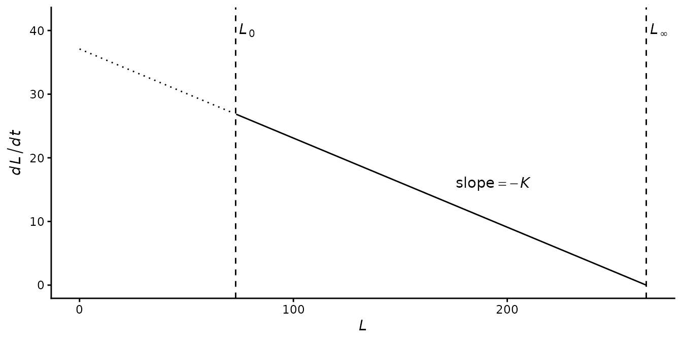
Figure 1. Growth rate, $dL/dt$, as a function of length, $L$, for values similar to those estimated for female blacktip sharks below ($L_0$ = 73 cm, $L_\infty$ = 265 cm, $K$ = 0.14). The dotted line extends the relationship below length at birth.

The solution to this equation most often used in fisheries science, popularised by Beverton and Holt (1957), gives length as a function of age, $a$:

$$L(a) = L_\infty\left(1 - e^{-K(a - t_0)}\right)$$

The third parameter, $t_0$, is the hypothetical age at which length would be zero. Many teleost fishes hatch as small larvae, and for these $t_0$ has no biological meaning. Chondrichthyans are born live or hatch from egg cases at a relatively large size, and for them length at age zero is meaningful: it is length at birth. The curve can be recast with length at birth, $L_0$, the y-intercept, in place of $t_0$, the x-intercept (Figure 2):

$$L(a) = L_0 + (L_\infty - L_0)\left(1 - e^{-Ka}\right)$$

growth() uses this form, as did Harry et al. (2019). The two forms give identical lengths at age, and either intercept can be calculated from the other, since $L_0 = L_\infty(1 - e^{K t_0})$ (Harry et al. 2022). Both forms, and the conversion between them, are derived step by step in the mathematical derivations vignette. For the curve in Figure 2, a length at birth of 73 cm corresponds to a $t_0$ of -2.3 years, a little over two years before birth. Holden (1974) suggested that $-t_0$ could be taken as the gestation period, on the assumption that embryos grow along the same curve as animals after birth, which gave a way of estimating $K$ for species that had not been aged (e.g. Francis 1981). Later comparisons with $K$ from age and growth studies showed little agreement, and the assumption about embryonic growth is unsupported for most species (Pratt and Casey 1990).

Figure 2. The relationship in Figure 1 expressed as length at age. The first form of the equation defines the curve by where it would cross zero length, $t_0$; the second by where it starts, at length at birth, $L_0$.

The equations above are deterministic. They describe the average length at age, not the lengths of individual animals. Estimating $L_\infty$, $K$ and $L_0$ means confronting the model with paired length at age data, and that requires some model of how individuals vary about the average. Growth curves are commonly fitted by nonlinear least squares regression of length on age (Harry et al. 2022). This has largely been a matter of statistical convenience, and it implicitly assumes that the observed length of animal $i$ is normally distributed about the curve with a constant standard deviation, $\sigma$:

$$l_i = L(a_i) + \epsilon_i, \qquad \epsilon_i \sim N(0, \sigma^2)$$

Under this assumption a newborn and a 20 year old animal are equally likely to differ from the average length for their age by any given amount. In practice length at age usually becomes more variable as animals get older and larger. A more realistic, but still simple, alternative is for the coefficient of variation to be constant, so that the standard deviation is proportional to expected length (Cope and Punt 2007; Restrepo et al. 2010):

$$l_i = L(a_i) + \epsilon_i, \qquad \epsilon_i \sim N(0, \sigma_i^2)$$

$$\sigma_i = CV_L \, L(a_i)$$

The standard deviation, $\sigma_i$, now differs between animals, and $CV_L$ is the coefficient of variation of length at age. Restrepo et al. (2010) arrived at this form by allowing asymptotic length to vary among individuals, following Kirkwood and Somers (1984). It is the form used by growth(), with $CV_L$ estimated along with the growth parameters.

Harry et al. (2019) extended this model in three ways, each of which is optional in growth() and can be used independently of the others.

Sexual dimorphism

Growth often differs between the sexes in fishes, and in sharks females are generally the larger sex. Cortés (2000) found that, on average, the maximum size of males was about 10% smaller than that of females, and that males had higher values of $K$, approaching their maximum size more quickly. This has been explained in part by the need for females to reach a larger size to carry their young (Cortés 2000), and the difference is most pronounced in live-bearing species (Gayford and Sternes 2024).

Differences in growth between the sexes are usually accommodated by fitting separate models to males and females. For data-limited species such as many elasmobranchs, this means that parameters such as $L_0$ and $\sigma$ are estimated separately when they could reasonably be shared. growth() is more parsimonious. It fits both sexes in a single model, with $L_\infty$ and $K$ estimated separately for each group, typically sex, while $L_0$ and $CV_L$ are shared:

$$L_g(a) = L_0 + (L_{\infty,g} - L_0)\left(1 - e^{-K_g a}\right)$$

Ageing error

Ages read from vertebrae are estimates, not measurements. Treating them as exact can bias growth estimates, by an amount that depends on how imprecise the readings are and where in the age range the error falls. The model treats true age as a random effect, with each reading an observation of it:

$$A_{i,j} = a_i + \epsilon_{a,ij}, \qquad \epsilon_{a,ij} \sim N(0, (CV_a a_i)^2)$$

The ageing CV is computed outside the likelihood from replicate readings, following Chang (1982), and held fixed.

Neonates

Animals with an unhealed umbilical scar are known to be age zero. Their lengths are direct information on $L_0$:

$$L_{0,i} \sim N(L_0, (CV_L L_{0,i})^2)$$

These are often available in numbers, and from animals that were never aged, so they add information at no cost.

Fitting is by maximum likelihood with RTMB, the random effects integrated out by the Laplace approximation. Confidence intervals on the curve come from the delta method; prediction intervals add $CV_L$.

This is a port of the TMB implementation used in Harry et al. (2019). The examples below use the data from that study.

Data

library(mustelus)
data(blacktip)

blacktip contains 475 common blacktip sharks, Carcharhinus limbatus, from south-east Queensland and northern New South Wales. Vertebrae were read by two readers for 102 sharks, all of them from New South Wales, where most sharks were caught on demersal setlines. A further 136 neonates with open or partially healed umbilical scars were sampled in Moreton Bay, Queensland. None of the neonates were aged. Length is stretched total length in cm.

Basic usage

g <- growth(STL, age_agree, sex, data = blacktip, neonate = neonate)
summary(g)
#> # A tibble: 2 × 17
#>   group  Linf Linf_lower Linf_upper     K K_lower K_upper    L0 L0_lower
#>   <chr> <dbl>      <dbl>      <dbl> <dbl>   <dbl>   <dbl> <dbl>    <dbl>
#> 1 f      265.       253.       276. 0.144   0.123   0.165  72.8     72.2
#> 2 m      242.       236.       248. 0.163   0.148   0.179  72.8     72.2
#> # ℹ 8 more variables: L0_upper <dbl>, CV_L <dbl>, n <int>, n0 <int>,
#> #   cv_age <dbl>, nll <dbl>, AIC <dbl>, convergence <lgl>

The summary has one row per group. $L_\infty$ and $K$ differ between them; $L_0$ and $CV_L$ are shared and so repeat. Also reported are the number of aged animals per group (n), the number of neonates (n0), the ageing CV if used, the negative log-likelihood, AIC, and whether the fit converged with a positive-definite Hessian.

Female blacktip sharks reach a larger asymptotic length than males (265 against 242 cm) and grow more slowly toward it (0.14 against 0.16). That pattern, females larger and slower, is common in carcharhinids.

Plotting

plot(g) + xlab("Age (years)") + ylab("Stretched total length (cm)")

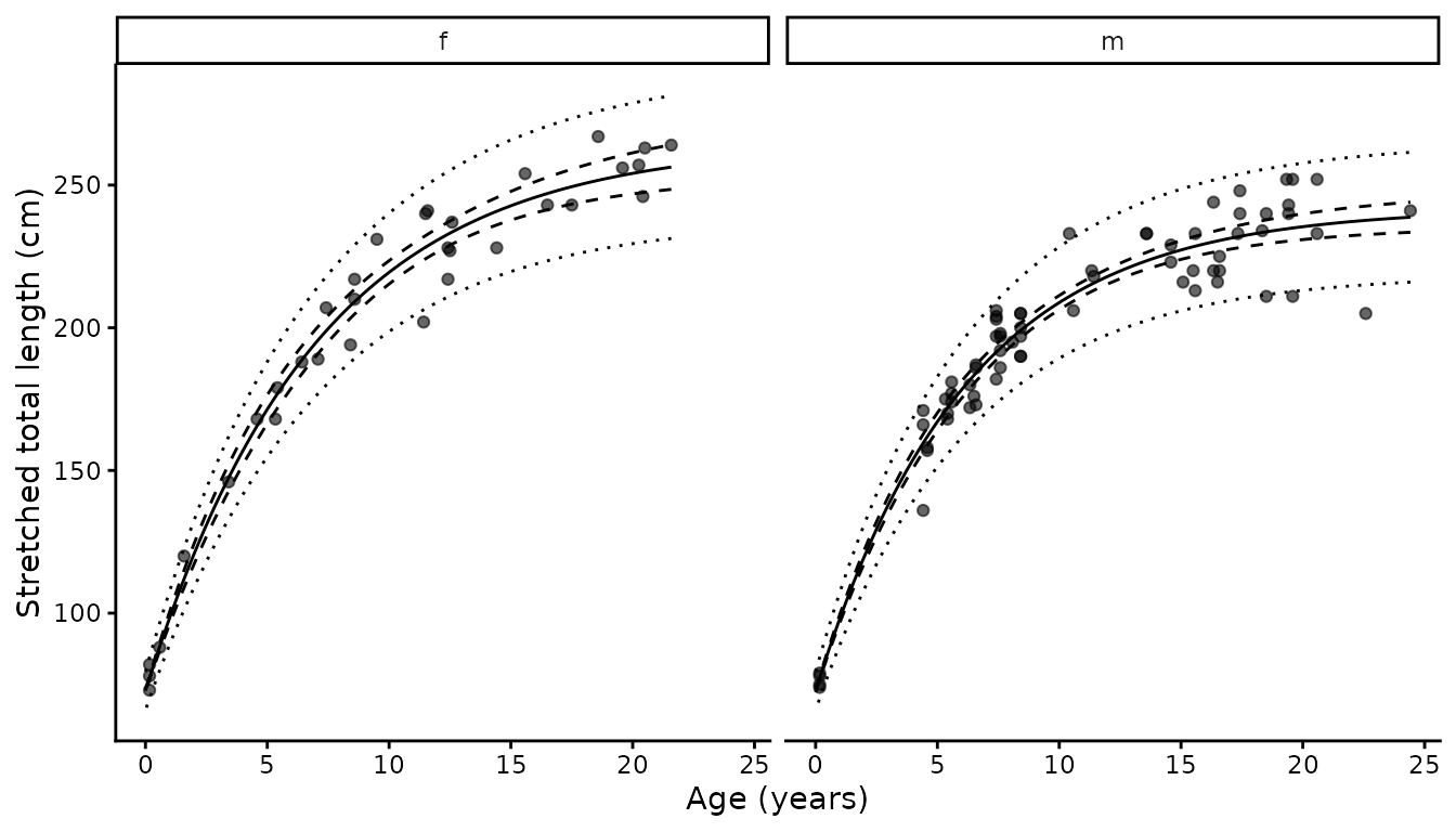
Figure 3. Length at age of female (f) and male (m) blacktip sharks with the fitted growth curves. The solid line is the fitted curve, the dashed ribbon the 95% confidence interval and the dotted ribbon the 95% prediction interval. Neonates, which inform $L_0$, are not shown.

In Figure 3 the solid line is the fitted curve, the dashed ribbon the 95% confidence interval on it, and the dotted ribbon the 95% prediction interval for individual animals. The prediction interval widens with size, which is the $CV_L$ assumption at work.

Comparing growth between sexes

$L_\infty$ and $K$ are estimated from the same data and are strongly correlated, -0.90 for females and -0.88 for males. A larger asymptote can be traded against slower growth toward it with little change in the fit. The confidence intervals reported for each parameter separately are therefore not a good basis for comparing groups, and a joint confidence region showing the combinations of the two that are consistent with the data is more informative.

Kimura (1980) constructed these regions from contours of the residual sum of squares, $S$, which for normally distributed errors are contours of equal likelihood. A combination of parameters lies inside the approximate 95% region if

$$S(L_\infty, K, t_0) \le \hat{S}\left(1 + \frac{p}{N - p} F_{p, N-p}(0.95)\right)$$

where $\hat{S}$ is the minimum, $N$ is the number of observations and $p = 3$ is the number of parameters. A region in three dimensions is hard to display, so Kimura conditioned on $t_0$ at its estimate and drew the two-dimensional cross-section for $L_\infty$ and $K$.

growth() maximises a likelihood rather than minimising a sum of squares, because the standard deviation changes with length. The same criterion in terms of the log-likelihood $\ell$ is

$$2\left[\hat{\ell} - \ell(L_\infty, K)\right] \le N \log\left(1 + \frac{p}{N - p} F_{p, N-p}(0.95)\right)$$

which for a single group with constant variance is identical to Kimura’s. growth_region() applies this criterion to a growth() fit. $L_0$ takes the place of $t_0$ and is held at its estimate, and $CV_L$ is re-estimated at each point, as $\sigma$ effectively is in the ratio of sums of squares. $N$ is the number of aged sharks of that sex. As in Kimura (1980), the boundary is found by stepping through values of $K$ and solving for the two values of $L_\infty$ at which the likelihood reaches the critical value.

r <- growth_region(g)
summary(r)
#> # A tibble: 2 × 9
#>   group  Linf Linf_min Linf_max     K K_min K_max     n level
#>   <chr> <dbl>    <dbl>    <dbl> <dbl> <dbl> <dbl> <int> <dbl>
#> 1 f      265.     250.     285. 0.144 0.116 0.178    33  0.95
#> 2 m      242.     233.     252. 0.163 0.142 0.187    69  0.95

summary() gives the estimates and the range of each parameter within the region.

plot(r) + labs(x = "Linf (cm)", y = "K (per year)", linetype = "Sex")

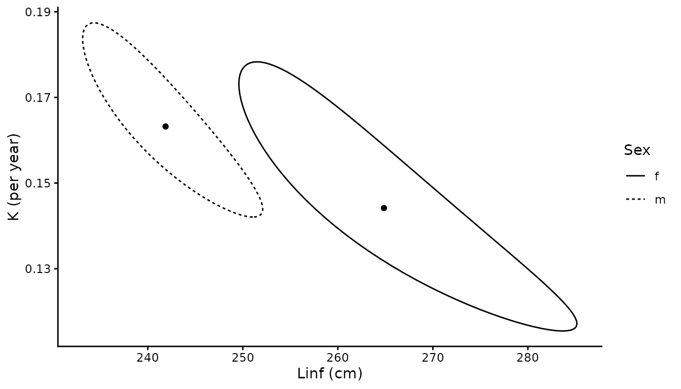
Figure 4. Approximate 95% joint confidence regions for $L_\infty$ and $K$ for female (f) and male (m) blacktip sharks, following Kimura (1980). Points are the maximum likelihood estimates.

The regions in Figure 4 are not symmetrical about the estimates, as an ellipse drawn from the covariance matrix would be. Each follows the curved ridge in the likelihood surface along which $L_\infty$ is traded against $K$, and extends further above the estimates than below them. For females the region reaches about 20 cm above the estimate of $L_\infty$ but only 15 cm below it. The intervals on $K$ alone overlap between the sexes (0.123 to 0.165 for females, 0.148 to 0.179 for males), but the two regions do not. Taken together, the two parameters describe clearly different growth curves for females and males.

As Kimura noted for $t_0$, holding $L_0$ fixed means these are cross-sections rather than true confidence regions, since more extreme values of $L_\infty$ and $K$ may occur at a different $L_0$. Setting profile_L0 = TRUE re-estimates $L_0$ at each point as well, giving the projection of the full three-parameter region. Here that makes almost no difference, because $L_0$ is closely determined by the neonates. Without neonates or young animals $L_0$ is poorly determined, and the projection can be noticeably wider, mainly in $K$.

growth_region() also works on models fitted with ageing error. Each evaluation of the likelihood then includes the Laplace approximation, so the calculation takes noticeably longer.

Length at birth

Supplying neonate flags animals of known age zero. Any flagged animal that also carries an age is used only for the length at birth term, not as length at age data: an age-zero observation and a length at birth observation say exactly the same thing, so counting both would double the weight. The function reports how many were moved.

In blacktip the neonates come from a separate sample, and the aged sharks include only 9 under two years old. Fitting the model without the neonates shows what they contribute:

g_no_neo <- growth(STL, age_agree, sex, data = blacktip)

rbind(
  with_neonates    = summary(g)[1, c("L0", "L0_lower", "L0_upper")],
  without_neonates = summary(g_no_neo)[1, c("L0", "L0_lower", "L0_upper")]
)
#> # A tibble: 2 × 3
#>      L0 L0_lower L0_upper
#> * <dbl>    <dbl>    <dbl>
#> 1  72.8     72.2     73.3
#> 2  72.6     69.8     75.4

The estimate of $L_0$ hardly changes, but the confidence interval is about five times narrower with the neonates included. Neonates are frequently the only data available for the smallest sizes.

Ageing error

Where replicate readings exist, pass the columns to reads and the ageing CV is computed from them. The readings need to be on the same scale as age. A reading is a count of growth zones and so is a whole number, but the ages in blacktip also include a fractional adjustment for the time elapsed since the population birth date of 1 November. That adjustment depends on the date of capture rather than on the reader, so it is the same for every reading of a given animal and is added to each one.

library(dplyr)

aged <- filter(blacktip, !is.na(age_agree))
table(difference = round(aged$reader2 - aged$reader1))
#> difference
#> -3 -2 -1  0  1  2  3  4 
#>  1  6 16 48 16  9  3  3

The two readers agreed on 48 of the 102 sharks. Most disagreements were of a single zone, and disagreement was far more common in sharks older than ten years. This is the usual pattern for vertebral ageing.

g_reads <- growth(STL, age_agree, sex, data = blacktip, neonate = neonate,
                  reads = c(reader1, reader2))
summary(g_reads)[, c("group", "Linf", "K", "L0", "cv_age")]
#> # A tibble: 2 × 5
#>   group  Linf     K    L0 cv_age
#>   <chr> <dbl> <dbl> <dbl>  <dbl>
#> 1 f      264. 0.142  72.8 0.0812
#> 2 m      242. 0.159  72.8 0.0812

The ageing CV is 8.1%. Compared with the fit that treats age as exact, $K$ falls by 1.5% for females and 2.6% for males, and $L_\infty$ moves by less than 1 cm. Both shifts are well inside the confidence intervals. Most of the disagreement between readers is in older sharks, where the curve is nearly flat and length says little about which reading is closer to the truth. The model treats the ages of those sharks as more uncertain, but does not move them much. With less precise ageing the effect can be considerably larger.

These estimates differ slightly from those published in Harry et al. (2019). The loop over readings in the original code started at the second reader, so the first reader’s counts were never used. Fitted to the second reader alone, growth() reproduces the published estimates to within rounding: $L_{\infty}$ 263.3 and 241.9 cm, $K$ 0.1418 and 0.1565, $L_0$ 72.77 cm and $CV_L$ 0.0487.

Leaving the birth date adjustment off the readings is an easy mistake to make. Here it gives the youngest sharks readings of zero, and growth() stops:

no_adj <- blacktip |>
  mutate(reader1 = floor(reader1), reader2 = floor(reader2))

growth(STL, age_agree, sex, data = no_adj, neonate = neonate,
       reads = c(reader1, reader2))
#> Error in `growth()`:
#> ! Ageing error needs every reading to be greater than zero. A reading of zero makes the likelihood unbounded, because the standard deviation of a reading is proportional to age. Add the birth date adjustment to each reading, and supply animals of known age zero through 'neonate'.

Because the standard deviation of a reading is proportional to age, a reading of zero can be explained exactly by a true age of zero, and the likelihood has no maximum. Where no readings are zero the model will fit, but the readings then sit below the true ages by the missing fraction, around half a year on average here, and the model treats every animal as younger than it is.

If only a consensus age is available but the ageing CV is known from elsewhere, supply it directly with cv_age. This is the more common situation when reanalysing published data.

g_cv <- growth(STL, age_agree, sex, data = blacktip, neonate = neonate,
               cv_age = 0.08)
summary(g_cv)[, c("group", "Linf", "K", "L0", "cv_age")]
#> # A tibble: 2 × 5
#>   group  Linf     K    L0 cv_age
#>   <chr> <dbl> <dbl> <dbl>  <dbl>
#> 1 f      280. 0.121  73.0   0.08
#> 2 m      265. 0.123  73.0   0.08

$K$ falls, as it did with the two readings, though by less. The two analyses are not equivalent, because the data going in are not the same. The consensus age matches the first reader’s count for 84 of the 102 sharks, and differs from the mean of the two readings for 46.

With neither reads nor cv_age, age is treated as measured without error and the model reduces to an ordinary von Bertalanffy fit.

Output structure

# Fixed-effect estimates and standard errors
summary(g$mods[[1]]$sdreport, "fixed")
#>          Estimate  Std. Error
#> Linf 264.84868596 5.928013298
#> Linf 241.86909868 3.274932763
#> K      0.14416127 0.010614934
#> K      0.16322060 0.007855840
#> L0    72.76498022 0.289193552
#> CV_L   0.04729473 0.002167525

head(g$preds[[1]])
#>   group       age       len    lower     upper   plower    pupper
#> 1     f 0.0000000  72.76498 72.19816  73.33180 65.99606  79.53390
#> 2     f 0.2180135  78.70811 77.96658  79.44965 71.37447  86.04176
#> 3     f 0.4360269  84.46737 83.33357  85.60117 76.55578  92.37896
#> 4     f 0.6540404  90.04843 88.49652  91.60033 81.55811  98.53874
#> 5     f 0.8720539  95.45680 93.50329  97.41032 86.39511 104.51850
#> 6     f 1.0900673 100.69785 98.36932 103.02638 91.07734 110.31835

mods holds the RTMB objective function, the nlminb result and the sdreport. Note that the objective is an external pointer and will not survive saveRDS(); the rest of the object is ordinary R data.

References

Beverton, R.J.H. and Holt, S.J. (1957) On the Dynamics of Exploited Fish Populations. Fishery Investigations Series II, Volume 19. Ministry of Agriculture, Fisheries and Food, London.

Chang, W.Y.B. (1982) A statistical method for evaluating the reproducibility of age determination. Canadian Journal of Fisheries and Aquatic Sciences 39(8), 1208–1210. doi:10.1139/f82-158

Cope, J.M. and Punt, A.E. (2007) Admitting ageing error when fitting growth curves: an example using the von Bertalanffy growth function with random effects. Canadian Journal of Fisheries and Aquatic Sciences 64(2), 205–218. doi:10.1139/f06-179

Cortés, E. (2000) Life history patterns and correlations in sharks. Reviews in Fisheries Science 8(4), 299–344. doi:10.1080/10641260008951115

Francis, M.P. (1981) Von Bertalanffy growth rates in species of Mustelus (Elasmobranchii: Triakidae). Copeia 1981(1), 189–192. doi:10.2307/1444053

Gayford, J.H. and Sternes, P.C. (2024) The origins and drivers of sexual size dimorphism in sharks. Ecology and Evolution 14(3), e11163. doi:10.1002/ece3.11163

Harry, A.V., Butcher, P.A., Macbeth, W.G., Morgan, J.A.T., Taylor, S.M. and Geraghty, P.T. (2019) Life history of the common blacktip shark, Carcharhinus limbatus, from central eastern Australia and comparative demography of a cryptic shark complex. Marine and Freshwater Research 70(6), 834–848. doi:10.1071/MF18141

Harry, A.V., Smart, J.J. and Pardo, S.A. (2022) Understanding the age and growth of chondrichthyan fishes. In: Carrier, J.C., Simpfendorfer, C.A., Heithaus, M.R. and Yopak, K.E. (eds) Biology of Sharks and Their Relatives, 3rd edn. CRC Press, Boca Raton, FL, pp. 177–202. doi:10.1201/9781003262190-6

Holden, M.J. (1974) Problems in the rational exploitation of elasmobranch populations and some suggested solutions. In: Harden Jones, F.R. (ed) Sea Fisheries Research. Halsted Press, John Wiley & Sons, New York, pp. 117–137.

Kimura, D.K. (1980) Likelihood methods for the von Bertalanffy growth curve. Fishery Bulletin 77(4), 765–776.

Kirkwood, G.P. and Somers, I.F. (1984) Growth of two species of tiger prawn, Penaeus esculentus and P. semisulcatus, in the western Gulf of Carpentaria. Australian Journal of Marine and Freshwater Research 35(6), 703–712. doi:10.1071/MF9840703

Pratt, H.L., Jr. and Casey, J.G. (1990) Shark reproductive strategies as a limiting factor in directed fisheries, with a review of Holden’s method of estimating growth-parameters. In: Pratt, H.L., Jr., Gruber, S.H. and Taniuchi, T. (eds) Elasmobranchs as Living Resources: Advances in the Biology, Ecology, Systematics, and the Status of the Fisheries. NOAA Technical Report NMFS 90, pp. 97–109. NOAA Technical Report NMFS 90

Restrepo, V.R., Diaz, G.A., Walter, J.F., Neilson, J.D., Campana, S.E., Secor, D. and Wingate, R.L. (2010) Updated estimate of the growth curve of Western Atlantic bluefin tuna. Aquatic Living Resources 23(4), 335–342. doi:10.1051/alr/2011004

von Bertalanffy, L. (1938) A quantitative theory of organic growth (inquiries on growth laws. II). Human Biology 10, 181–213.