Analyse growth from length at age data

Fits a von Bertalanffy growth model to length at age data, following Harry et al. (2019), which builds on Cope and Punt (2007). The curve is parameterised by length at birth rather than $t_0$:

Usage

growth(
  len,
  age,
  grouping_var = NULL,
  data,
  neonate = NULL,
  reads = NULL,
  cv_age = NULL,
  start = NULL
)

Arguments

len: Numeric vector of lengths
age: Numeric vector of ages. Used directly when ageing error is off, and as the starting value for true age when it is on.
grouping_var: Optional grouping variable (typically sex). Separate Linf and K are estimated per group; L0 and CV_L are shared.
data: A data frame containing the above variables
neonate: Optional indicator for individuals of known age zero. Anything coercible to logical, e.g. umb_scar %in% c("y", "p").
reads: Optional replicate age reading columns, e.g. c(reader1, reader2). Switches on ageing error. Readings must be on the same scale as age: where ages include an adjustment for birth date, the same adjustment should be added to each reading. Readings must be greater than zero.
cv_age: Optional ageing CV supplied directly. An alternative to reads when only a consensus age is available.
start: Optional named list of starting values for Linf, K, L0 and CV_L. Derived from the data if NULL.

Value

A one row tibble of class "growth" containing the list columns data, coefs, preds, mods and neonates. coefs has one row per group, with L0 and CV_L repeated since they are shared. mods holds the RTMB objective, the nlminb result and the sdreport.

Details

$$L_{i,g}(a) = L_0 + (L_{\infty,g} - L_0)(1 - e^{-K_g a_{i,g}})$$

where $L_{\infty,g}$ and $K_g$ may differ between groups (typically sexes) while $L_0$ is shared. Observed length is normally distributed about the curve with a standard deviation proportional to expected length, $\sigma_{L} = CV_L L_{i,g}$, so variability in length at age grows with size.

Two optional extensions from the paper can each be switched on independently.

Ageing error. Supplying reads, two or more columns of replicate age readings, treats true age as a random effect. Observed readings are linked to true age by $A_{i,j} = a_i + \epsilon$, with $\epsilon \sim N(0, (CV_a a_i)^2)$. The ageing CV is computed from the replicate readings outside the likelihood and held fixed. Alternatively cv_age supplies that CV directly, which is useful where only a consensus age is available but the ageing CV is known from elsewhere. With neither argument, age is treated as measured without error.

Neonates. Supplying neonate, an indicator for individuals of known age zero such as those with an unhealed umbilical scar, adds their lengths as direct information on $L_0$ through $L_{0,i} \sim N(L_0, (CV_L L_{0,i})^2)$. Flagged individuals are used only for this term: any that also carry an age are removed from the length at age data, since an age-zero observation and a length at birth observation carry the same information and including both would count it twice.

Estimation is by maximum likelihood using RTMB, with the random effects integrated out by the Laplace approximation. Confidence intervals on the fitted curve come from the delta method via sdreport; prediction intervals add the individual variability $CV_L$.

References

Cope, J.M. and Punt, A.E. (2007) Admitting ageing error when fitting growth curves: an example using the von Bertalanffy growth function with random effects. Canadian Journal of Fisheries and Aquatic Sciences 64(2), 205-218. doi:10.1139/f06-179

Harry, A.V., Butcher, P.A., Macbeth, W.G., Morgan, J.A.T., Taylor, S.M. and Geraghty, P.T. (2019) Life history of the common blacktip shark, Carcharhinus limbatus, from central eastern Australia and comparative demography of a cryptic shark complex. Marine and Freshwater Research 70(6), 834-848. doi:10.1071/MF18141

Examples

library(ggplot2)
data(spottail)

# Sex-specific growth, with neonates informing length at birth
g <- growth(length, age_agree, sex, data = spottail,
            neonate = umb_scar %in% c("y", "p"))
#> The categorical variable sex has 2 levels.
#> 5 neonate(s) with an age were used only for length at birth, not as length at age data.

summary(g)
#> # A tibble: 2 × 17
#>   group  Linf Linf_lower Linf_upper     K K_lower K_upper    L0 L0_lower
#>   <chr> <dbl>      <dbl>      <dbl> <dbl>   <dbl>   <dbl> <dbl>    <dbl>
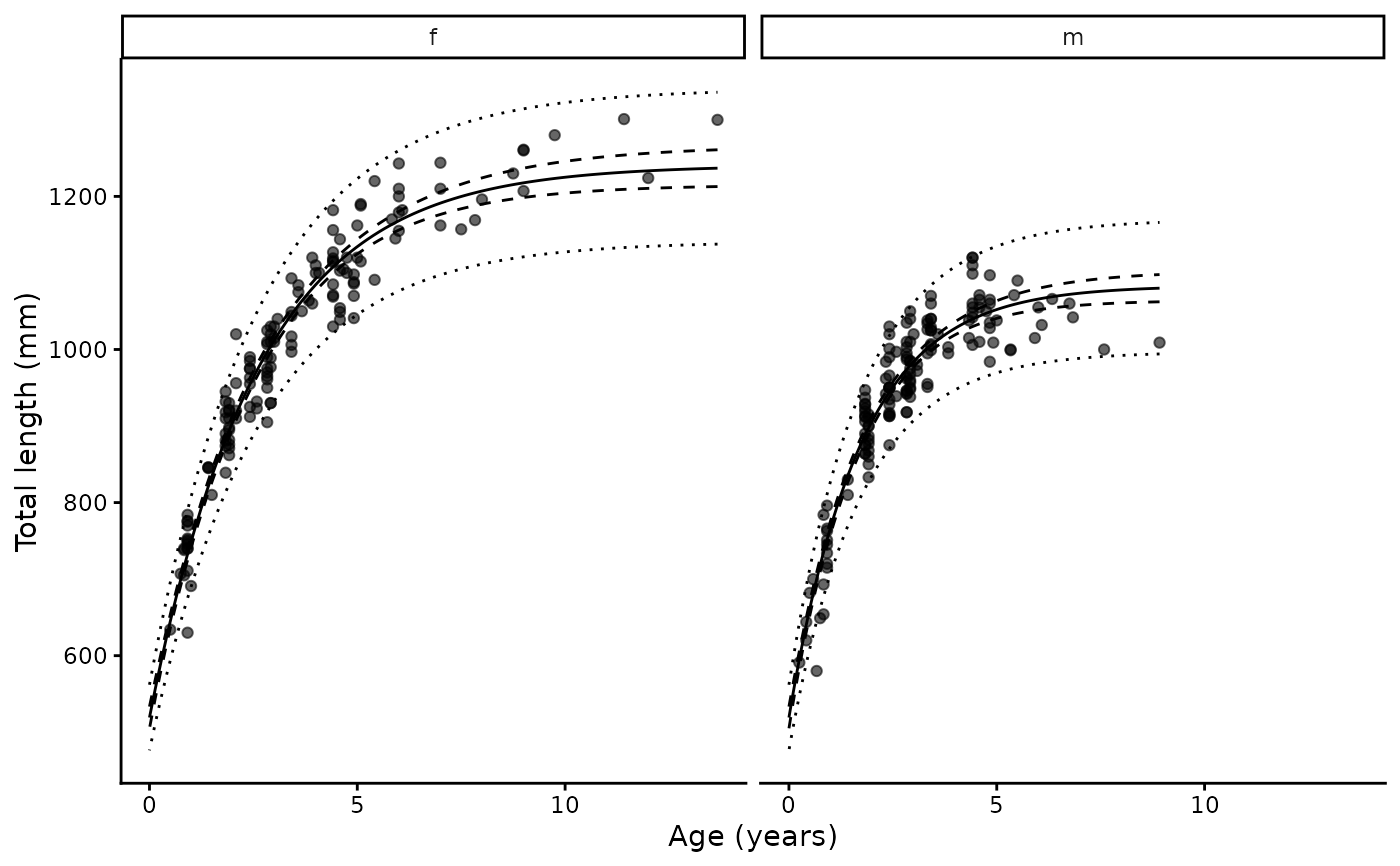
#> 1 f      1241       1215       1266 0.383   0.350   0.415  519.     505.
#> 2 m      1083       1064       1103 0.580   0.526   0.633  519.     505.
#> # ℹ 8 more variables: L0_upper <dbl>, CV_L <dbl>, n <int>, n0 <int>,
#> #   cv_age <dbl>, nll <dbl>, AIC <dbl>, convergence <lgl>

plot(g) + xlab("Age (years)") + ylab("Total length (mm)")


# Ageing error from two readers, as in Harry et al. (2019)
data(blacktip)
g2 <- growth(STL, age_agree, sex, data = blacktip, neonate = neonate,
             reads = c(reader1, reader2))
#> The categorical variable sex has 2 levels.
#> Ageing CV computed from 2 readings: 0.0812.

summary(g2)
#> # A tibble: 2 × 17
#>   group  Linf Linf_lower Linf_upper     K K_lower K_upper    L0 L0_lower
#>   <chr> <dbl>      <dbl>      <dbl> <dbl>   <dbl>   <dbl> <dbl>    <dbl>
#> 1 f      264.       252.       276. 0.142   0.120   0.164  72.8     72.2
#> 2 m      242.       236.       249. 0.159   0.143   0.175  72.8     72.2
#> # ℹ 8 more variables: L0_upper <dbl>, CV_L <dbl>, n <int>, n0 <int>,
#> #   cv_age <dbl>, nll <dbl>, AIC <dbl>, convergence <lgl>