Length at maturity analysis • mustelus

The maturity() function fits a logistic regression of binary maturity (0 = immature, 1 = mature) as a function of a continuous predictor such as length or age:

$P(\text{mature}) = \frac{1}{1 + e^{-(a + b \cdot L)}}$

Key outputs are $L_{50}$ and $L_{95}$ — the lengths (or ages) at which 50% and 95% of individuals are expected to be mature — with bootstrap confidence intervals.

Basic usage

library(mustelus)
#> Welcome to mustelus package
data(spottail)

lm50 <- maturity(maturity_stage, length, data = spottail, times = 200)
summary(lm50)
#> # A tibble: 1 × 10
#>       a      b   L50 L50_lower L50_upper   L95 L95_lower L95_upper     n     N
#>   <dbl>  <dbl> <dbl>     <dbl>     <dbl> <dbl>     <dbl>     <dbl> <int> <int>
#> 1 -55.4 0.0594  934.      926.      942.  983.      965.      1002   430   341

Grouping by sex

lm50_sex <- maturity(maturity_stage, length, sex, data = spottail, times = 200)
#> The categorical variable sex has 2 levels.
#> Warning: There was 1 warning in `mutate()`.
#> ℹ In argument: `.fit = map(data, ~maturity_mod(.x))`.
#> ℹ In group 2: `grouping_var = "f"`.
#> Caused by warning:
#> ! glm.fit: fitted probabilities numerically 0 or 1 occurred
summary(lm50_sex)
#> # A tibble: 3 × 10
#>        a      b   L50 L50_lower L50_upper   L95 L95_lower L95_upper     n     N
#>    <dbl>  <dbl> <dbl>     <dbl>     <dbl> <dbl>     <dbl>     <dbl> <int> <int>
#> 1  -55.4 0.0594  934.      926.      942.  983.      963.      998.   430   341
#> 2 -124.  0.131   951.      940.      965.  973.      942.      993.   118    97
#> 3  -51.1 0.0550  929.      920.      940.  983.      963.     1002    312   244

Plotting

plot() returns a named list of ggplot objects. The default shows binned observed proportions scaled by sample size, as for females in Figure 1.

p <- plot(lm50_sex)
p$f + xlab("Total length (mm)") + ylab("Proportion mature")

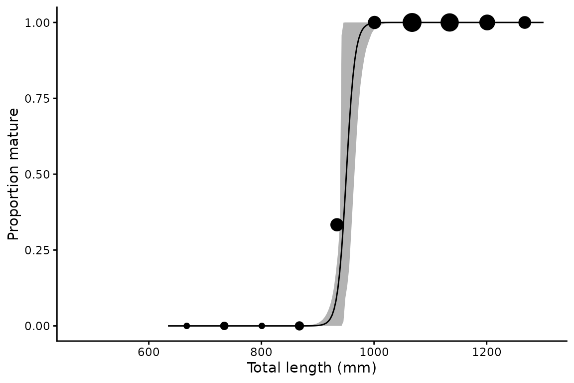
Figure 1. Proportion mature against total length for female spot-tail sharks, with the fitted logistic curve and its bootstrap 95% confidence interval (grey ribbon). Points are observed proportions in length bins, sized by the number of animals in each bin.

Plot styles

Three styles for raw data display are available, shown for both sexes combined in Figure 2 to Figure 4:

# Proportions (default) — point size scaled by n per bin
plot(lm50, raw_data = "proportions")$Unspecified +
  xlab("Total length (mm)") + ylab("Proportion mature")

Figure 2. Proportion mature against total length for spot-tail sharks of both sexes combined, with points sized by the number of animals in each bin (the default). Curve and ribbon as in Figure 1.

# Point — same bins, uniform point size
plot(lm50, raw_data = "point")$Unspecified +
  xlab("Total length (mm)") + ylab("Proportion mature")

**Figure 3.** As [Figure 2](#mat-proportions), with points of uniform size.

Figure 3. As Figure 2, with points of uniform size.

# Rug — mature individuals on top, immature on bottom
plot(lm50, raw_data = "rug")$Unspecified +
  xlab("Total length (mm)") + ylab("Proportion mature")

**Figure 4.** As [Figure 2](#mat-proportions), with individual animals shown as a rug, mature animals along the top axis and immature animals along the bottom.

Figure 4. As Figure 2, with individual animals shown as a rug, mature animals along the top axis and immature animals along the bottom.

Adjusting bin width

The binwidth argument controls the width of bins in data units (default is range/10). Figure 5 uses 50 mm bins:

plot(lm50, binwidth = 50)$Unspecified +
  xlab("Total length (mm)") + ylab("Proportion mature")

**Figure 5.** As [Figure 2](#mat-proportions), with 50 mm bins.

Figure 5. As Figure 2, with 50 mm bins.

Using age as the predictor

maturity() works with any continuous predictor — here using age rather than length:

am50 <- maturity(maturity_stage, age_agree, data = spottail, times = 200)
#> Warning: There was 1 warning in `mutate()`.
#> ℹ In argument: `.fit = map(data, ~maturity_mod(.x))`.
#> ℹ In group 1: `grouping_var = Unspecified`.
#> Caused by warning:
#> ! glm.fit: fitted probabilities numerically 0 or 1 occurred
summary(am50)
#> # A tibble: 1 × 10
#>       a     b   L50 L50_lower L50_upper   L95 L95_lower L95_upper     n     N
#>   <dbl> <dbl> <dbl>     <dbl>     <dbl> <dbl>     <dbl>     <dbl> <int> <int>
#> 1 -9.50  4.05  2.35      2.19      2.48  3.07      2.62      3.38   211   153

The fitted ogive is shown in Figure 6.

plot(am50, binwidth = 1)$Unspecified +
  xlab("Age (years)") + ylab("Proportion mature")

Figure 6. Proportion mature against age for spot-tail sharks of both sexes combined, in 1 year bins. Curve and ribbon as in Figure 1.

Output structure

Like len_weight(), the result is a nested tibble with named list columns per group:

# Bootstrap L50 estimates for all individuals
quantile(lm50_sex$mods[["f"]]$fitted.values)
#>           0%          25%          50%          75%         100% 
#> 2.220446e-16 9.986775e-01 1.000000e+00 1.000000e+00 1.000000e+00

# Predicted maturity curve for females
head(lm50_sex$preds[["f"]])
#>          x          mat        lower        upper
#> 1 634.0000 2.220446e-16 2.220446e-16 5.346166e-13
#> 2 637.3518 2.220446e-16 2.220446e-16 7.193201e-13
#> 3 640.7035 2.220446e-16 2.220446e-16 9.678395e-13
#> 4 644.0553 2.220446e-16 2.220446e-16 1.302224e-12
#> 5 647.4070 2.220446e-16 2.220446e-16 1.752143e-12
#> 6 650.7588 2.220446e-16 2.220446e-16 2.357515e-12