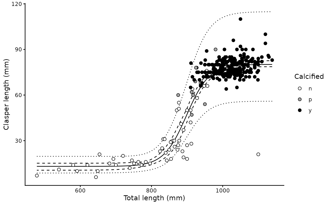
Fits a nonlinear (logistic) model of clasper length against a continuous predictor such as body length or age, describing the rapid elongation of claspers that accompanies maturation in male chondrichthyans. The model is
Arguments
- clasp
Numeric vector of clasper lengths
- x
Continuous predictor variable (e.g. length, age)
- calc
Optional clasper calcification stage, conventionally coded
"n"(not calcified),"p"(partially calcified) and"y"(calcified). Used only for plotting, where points are shaded white, grey and black respectively; it does not enter the model.- data
A data frame containing the above variables
- times
Number of bootstrap replicates (default 1000)
- start
Optional named list of starting values for
a,b,L50andL95. IfNULL(the default) these are derived from the data.
Value
A one row tibble of class "clasp_length" containing the list
columns data, coefs, preds, mods and
boot_coefs.
Details
$$CL = b + (a - b)\left(1 + e^{-\log(19)(x - L_{50})/(L_{95} - L_{50})}\right)^{-1}$$
where b and a are the juvenile and adult asymptotes, and
L50 and L95 are the values of the predictor at which clasper
length reaches 50 and 95 percent of the way between them. It is fitted on the
log scale via nls(), giving multiplicative error, so the fitted curve
describes median rather than mean clasper length.
Confidence intervals on the parameters and on the fitted curve are obtained by
bootstrap resampling with rsample. Prediction intervals combine the
bootstrap variance of the curve with the residual variance of the fit.
Records with missing or non-positive clasper length are dropped, so passing a
data frame containing both sexes is safe provided females are recorded as
NA.
Examples
library(ggplot2)
data(spottail)

cl <- clasp_length(clasp_length, length, clasp_calc, data = spottail, times = 200)
#> The calcification variable clasp_calc has 3 levels.

summary(cl)
#> # A tibble: 1 × 15
#>       a a_lower a_upper     b b_lower b_upper   L50 L50_lower L50_upper   L95
#>   <dbl>   <dbl>   <dbl> <dbl>   <dbl>   <dbl> <dbl>     <dbl>     <dbl> <dbl>
#> 1  80.2    78.7    82.7  13.1    10.6    15.2  898.      889.       908  992.
#> # ℹ 5 more variables: L95_lower <dbl>, L95_upper <dbl>, Sigma <dbl>, n <int>,
#> #   x.range <chr>

plot(cl) + xlab("Total length (mm)") + ylab("Clasper length (mm)")